Filtering with low, band and high-pass filters

In this notebook, we will create ideal low-pass, high-pass and band-pass filters, and apply them to a signal to study their effects.

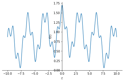
Let us first create a signal with multiple frequency components. For example, a continuous time signal with three different frequencies combined:

\[ x(t) = \cos(0.1 t) + 0.5 \cos(2 t) + 0.2\cos(7 t). \]

This signal has three different frequencies: a low frequency \(\omega_0=0.1\), a middle frequency \(\omega_0 = 2\) and a high frequency \(\omega_0 = 7\). Note that there is no absolute criterion to name a frequency as low, mid or high. We use them relatively.

Let us define this function in SymPy and plot it.

import sympy as sym
    
sym.init_printing()

t = sym.symbols('t', real=True)

x = sym.cos(0.1*t) + 0.5*sym.cos(2*t) + 0.2*sym.cos(7*t)

sym.plot(x, (t,-10,10));

What is the Fourier transform of this signal? We know that

\[ \cos(\omega_0 t) \overset{F.T.}{\longleftrightarrow} \pi \left( \delta(\omega-\omega_0) + \delta(\omega+\omega_0) \right) \]

Using the linearity property of Fourier transform, we can conclude that the Fourier transform of \(x(t)\) is

\[ x(t) \overset{F.T.}{\longleftrightarrow} \pi \left( \delta(\omega-0.1) + \delta(\omega+0.1) + 0.5\delta(\omega-2) + 0.5\delta(\omega+2) + 0.2\delta(\omega-7) + 0.2\delta(\omega+7)\right) \]

We can validate this by computing the Fourier transform using SymPy as follows

from sympy import I # the imaginary number "j" is represented as "I" in SymPy
omega = sym.symbols('omega', real=True)
X = sym.integrate(x*sym.exp(-I*omega*t), (t, -sym.oo, sym.oo))
sym.simplify(X)

\[\begin{split}\displaystyle \begin{cases} \frac{i \omega \left(2.22044604925031 \cdot 10^{-16} - 1.4210854715202 \cdot 10^{-14} \omega^{2}\right)}{\left(\omega^{2} - 0.01\right) \left(100.0 \omega^{2} - 1\right)} & \text{for}\: \left|{2 \arg{\left(\omega \right)} - \pi}\right| < \pi \wedge \left|{2 \arg{\left(\omega \right)} + \pi}\right| < \pi \\\int\limits_{-\infty}^{\infty} \left(\cos{\left(0.1 t \right)} + 0.5 \cos{\left(2 t \right)} + 0.2 \cos{\left(7 t \right)}\right) e^{- i \omega t}\, dt & \text{otherwise} \end{cases}\end{split}\]

However, as you can see the output is not quite right. In fact, there is a known issue with SymPy about this at https://github.com/sympy/sympy/issues/2803. So, we write the Fourier transform of \(x(t)\) manually:

X = sym.pi*(sym.DiracDelta(omega-0.1)+sym.DiracDelta(omega+0.1)+ 
            0.5*sym.DiracDelta(omega-2)+0.5*sym.DiracDelta(omega+2)+
            0.2*sym.DiracDelta(omega-7)+0.2*sym.DiracDelta(omega+7) )
X

Next, we want to filter this signal with ideal low-pass, band-pass and high-pass filters.

Let us create these filters.

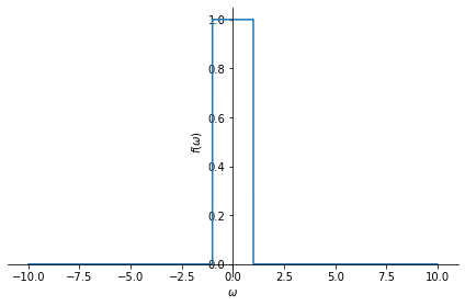
Ideal low-pass filter:

LP = sym.Heaviside(omega+1)-sym.Heaviside(omega-1)
sym.plot(LP, (omega, -10,10 ));

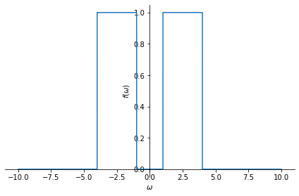
Ideal band-pass filter:

BP = sym.Heaviside(omega-1)-sym.Heaviside(omega-4) + sym.Heaviside(omega+4)-sym.Heaviside(omega+1)
sym.plot(BP, (omega, -10,10 ));

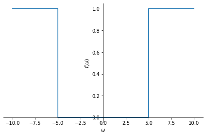
Ideal high-pass filter:

HP = -sym.Heaviside(omega+5)+sym.Heaviside(omega-5)+1
sym.plot(HP, (omega, -10,10 ));

Now let use apply the low-pass filter to \(x(t)\). We can do this application in two ways: 1) convolve them in the time domain, or 2) multiply them in the frequency domain. Since we already have the frequency domain representations of both the signal and the filter, we will follow the second method.

Let us apply the low-pass filter and do inverse Fourier transform on the result to obtain the time domain representation of the result:

y = (1/(2*sym.pi))*sym.integrate(X*LP*sym.exp(I*omega*t), (omega, -sym.oo, sym.oo))
sym.simplify(y)

Low-pass filtering gave use the low-frequency component of \(x(t)\).

Now let us apply the band-pass filter.

y = (1/(2*sym.pi))*sym.integrate(X*BP*sym.exp(I*omega*t), (omega, -sym.oo, sym.oo))
sym.simplify(y)

which correctly gave us the mid frequency component.

And, high-pass filtering will yield the high-frequency component of \(x(t)\):

y = (1/(2*sym.pi))*sym.integrate(X*HP*sym.exp(I*omega*t), (omega, -sym.oo, sym.oo))
sym.simplify(y)

In this notebook, we have seen a simple example of filtering. Our previous two notebooks also showcase filtering applications, one of them on 1D signals and the other on 2D signals.