How to reconstruct a 2D image using only sine functions

In the previous notebook, we decomposed a one dimensional signal into its frequency components using the Discrete Time Fourier Transform (DTFT) and the Discrete Time Fourier Transform (DFT). Here in this notebook, we will do a similar analysis on 2D signals. We will decompose a 2D signal into its frequency components and reconstruct it back.

2D DTFT

Remember the analysis equation of DTFT:

\[ \quad X(e^{j\omega}) = \sum_{n=-\infty}^{\infty}x[n]e^{-j\omega n}. \]

For 2D, this equation becomes the following:

\[ \quad X(e^{ju}, e^{jv}) = \sum_{m=-\infty}^{\infty} \sum_{n=-\infty}^{\infty}x[m,n]e^{-ju m - jvn}. \]

The implementation is straightforward (see the 1D DTFT implementation in the previous notebook) and left to the reader as exercise.

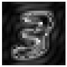
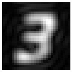
We are interested in applying the analysis equation to an image like this

This is an image from the MNIST dataset, which you might remember from the notebook An application of convolution in machine learning. It is a 28-by-28 pixel, grayscale image. It is a spatially limited signal, that is, it does not have any values outside the 28-by-28 area. However, the DTFT is for analyzing signals that extend from minus infinity to plus infinity. So, it can be represented as a 2D discrete time signal \(x[m,n]\) where the image pixels are embedded at \(0 \le m \le 27\) and \(0 \le n \le 27\); for all other locations (i.e. \(m<0\;\text{or}\; m>27\;\text{or}\;n<0\;\text{or}\;n>27\)), \(x[m,n]\) is zero.

The other alternative for applying Fourier transform on this image is to use the Discrete Fourier Transform (DFT), which is suitable for time limited or spatially limited data such as images.

2D DFT

The analysis equation for 2D DFT is as follows:

\[ X[u,v] = \sum_{m=0}^{M-1}\sum_{n=0}^{N-1} x[m,n] e^{-j 2 \pi (\frac{m}{M}u + \frac{n}{N} v)}. \]

2D DFT is implemented in numpy’s fft2. FFT stands for Fast Fourier Transform, which is a fast algorithm to compute DFT. The complex exponential in the right hand side represents waves of different frequencies and different orientations. To see this, let us plot its real part for some parameters. Remember that the Euler equation expands a complex exponential into sine and cosine waves: \(e^{j\theta} = \cos(\theta) + j\sin(\theta)\). So, the real part of the complex exponential above is \(\cos(2\pi (\frac{m}{M}u + \frac{n}{N} v))\). Below we create and plot cosine waves for different \(u\) and \(v\).

import numpy as np
from matplotlib import pyplot as plt 

def generate_wave(u,v):
    nrows = 50
    ncols = 50
    wave = np.zeros((nrows,ncols), dtype=np.float64)
    for m in range(nrows):
        for n in range(ncols):
            f = np.cos(2*np.pi*(u*m/nrows +v*n/ncols))
            wave[m,n] = np.abs(f)
    return wave

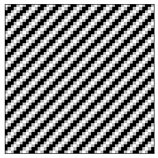
plt.imshow(generate_wave(5,5), cmap='gray');
plt.xticks([]), plt.yticks([]);

plt.imshow(generate_wave(0,3), cmap='gray');
plt.xticks([]), plt.yticks([]);

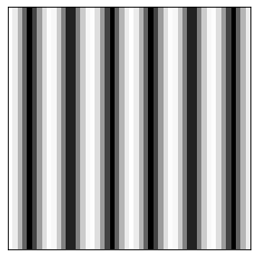
You are encouraged to play with the values of u and v above to see how the orientation and frequency of the wave changes.

Now let us apply 2D DFT to a simple image, an image of a white square on a black background as seen below.

image = np.zeros((13,13))
image[4:9,4:9] = 1
plt.imshow(image, cmap='gray')
plt.xticks([]), plt.yticks([]);

Below two lines compute the DFT of this image. Adn, we plot the magnitude spectrum.

ft = np.fft.fft2(image)
ft = np.fft.fftshift(ft)
plt.imshow(np.abs(ft), cmap='gray')
plt.xticks([]), plt.yticks([]);

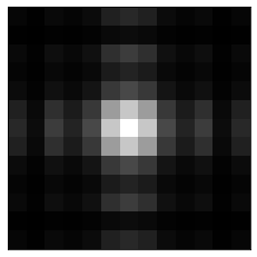
The second line above (the fftshift) shifts the zero-frequency component to the center of the spectrum. Thw low frequency components are around the center and the frequency gets higher as you move away from the center.

We can reconstruct back the original image from its Fourier transsform as follows.

recons_image = np.fft.ifft2(ft)
plt.imshow(np.abs(recons_image), cmap='gray')
plt.xticks([]), plt.yticks([]);

Now we will do another reconstruction but this time we will use only the low frequency components. We can achieve this by multiplying the Fourier transform with a mask as follows.

nrows, ncols = image.shape

# Build a mask 
x = np.linspace(0, nrows, nrows)
y = np.linspace(0, ncols, ncols)
X, Y = np.meshgrid(x, y)
cy, cx = nrows/2, ncols/2
mask = np.sqrt((X-cx)**2+(Y-cy)**2)
mask[mask<=4] = 1
mask[mask>4] = 0

plt.imshow(mask, cmap='gray')
plt.xticks([]), plt.yticks([]);

To form the mask we computed distances of each pixel from the center and then thresholded these distances with 4. Those loxations (pixels) that have a distance equal to or less than 4 is made 1, others 0. Now we can use this mask to reconstruct our image back by using only the low frequencies that correspond to the locations with mask value 1.

recons_image = np.fft.ifft2(ft*mask)
plt.imshow(np.abs(recons_image), cmap='gray')
plt.xticks([]), plt.yticks([]);

This result shows that when we use only the low frequency components, the reconstruction is blurry. We do not see the sharp edges of the square, as expected. Low frequency waves cannot reconstruct a sharp edge.

Now let us reverse the mask:

mask2 = mask.copy()
mask2[mask==1] = 0
mask2[mask==0] = 1
plt.imshow(mask2, cmap='gray')
plt.xticks([]), plt.yticks([]);

When we apply this mask to the Fourier transform and reconstruct the image, we only get the edges of the white square. This is expected because how we are using only the high frequency components which are good for reconstructing edges, i.e. sharp transitions.

recons_image = np.fft.ifft2(ft*mask2)
plt.imshow(np.abs(recons_image), cmap='gray')
plt.xticks([]), plt.yticks([]);

You are encouraged to play with the threshold value (4) of the mask above and see how it changes the reconstructions with the mask.

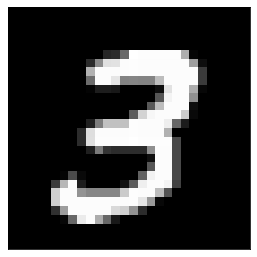
Now let us apply DFT to a real image. We will use an MNIST image:

from PIL import Image
import requests
from io import BytesIO

response = requests.get('https://384book.net/_images/3.png')
image = Image.open(BytesIO(response.content))
image = np.asarray(image)
image = image[:,:,0]

plt.imshow(image, cmap='gray')
plt.xticks([]), plt.yticks([]);

Here is how its DFT magnitude spectrum looks like:

ft = np.fft.fft2(image)
ft = np.fft.fftshift(ft)
plt.imshow(np.abs(ft), cmap='gray');
plt.xticks([]), plt.yticks([]);

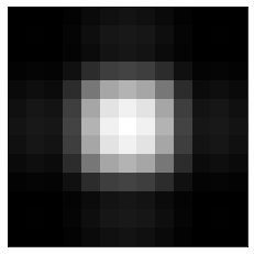
If we apply a mask to this spectrum to keep the low frequency components only, we get back a blurry “3”:

nrows, ncols = image.shape

# Build a mask 
x = np.linspace(0, nrows, nrows)
y = np.linspace(0, ncols, ncols)
X, Y = np.meshgrid(x, y)
cy, cx = nrows/2, ncols/2
mask = np.sqrt((X-cx)**2+(Y-cy)**2)
mask[mask<=4] = 1
mask[mask>4] = 0

plt.imshow(mask, cmap='gray')
plt.xticks([]), plt.yticks([]);

recons_image = np.fft.ifft2(ft*mask)
plt.imshow(np.abs(recons_image), cmap='gray')
plt.xticks([]), plt.yticks([]);

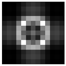
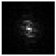
In contrast, if we adjust the mask so that it zeros out the low frequency components and keep only the high frequency components, we get the edges in the image:

mask2 = mask.copy()
mask2[mask==1] = 0
mask2[mask==0] = 1
plt.imshow(mask2, cmap='gray')
plt.xticks([]), plt.yticks([]);

recons_image = np.fft.ifft2(ft*mask2)
plt.imshow(np.abs(recons_image), cmap='gray')
plt.xticks([]), plt.yticks([]);