An example application: removing unwanted noise from audio

In this notebook, we will analyze sound waves in the frequency domain. We will demonstrate how modifying signals in the frequency domain can effectively “purify” them.

For frequency domain analysis, we will begin by examining the Discrete-Time Fourier Transform (DTFT). However, we will find that the DTFT is not very suitable for our purposes. The DTFT analyzes signals that exist across the entire time axis, extending from negative infinity to positive infinity. Since in this task we are dealing with practical signals that have a finite duration, the DTFT’s assumption of infinite signal length is not realistic.

To overcome this limitation, we will introduce the Discrete Fourier Transform (DFT). The DFT performs a frequency domain analysis similar to the DTFT, but specifically for signals that are time-limited. This makes it a more practical tool for our denoising task in this notebook.

Let us create an A4 tone, which has 440 Hz (cycles/second) frequency. It is the A above middle C in the piano. It is also the dial tone used in our phones.

import numpy as np

sampleRate = 24000 # samples per second
frequency = 440    # this is the frequency of note A4
duration = 1       # a second

n = np.linspace(0, duration, int(sampleRate * duration))  
x = np.sin(frequency * 2 * np.pi * n)  #  Has frequency of 440Hz   

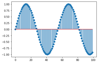
Here we created a signal in the form \(x[n] = sin(2\pi f n)\), where \(f\) is the frequency of the signal in cycles per second, or Hertz (Hz). The sample rate defines how many times per second a continuous signal is measured to create a digital representation. The value we use here (\(24000\)) is a typical value for audio WAV files.

Here is how the signal looks like:

from matplotlib import pyplot as plt
plt.stem(x[:100]); # we are just plotting the first 100 samples for visibility

And, here is how this signals sounds:

import sounddevice as sd
sd.play(x, sampleRate) 

Now let us pollute this nice tone with another high-pitch tone and with some random noise. For this, we will create a very high frequency signal and add normal random noise to it:

noise_freq = 7902 # this is the note B8
noise = 0.3*np.sin(noise_freq * 2 * np.pi * n) + 0.1*np.random.normal(0,1,len(x)) #  Has frequency of 440Hz

plt.stem(noise[:100])

<StemContainer object of 3 artists>

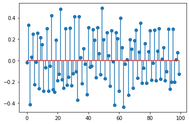
Here is how this signal sounds:

sd.default.reset()
sd.play(noise, sampleRate) 

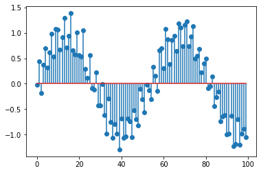
Now we create the polluted signal by adding the A4 tone with the noise we just created. Below we both plot and play it. Together with the A4 tone, you should be able to hear the high-pitch tone and a noisy “hiss” sound.

y = x + noise 

plt.stem(y[:100]);

sd.play(y)

One can develop a time-domain algorithm to smooth this polluted signal, that is, to remove both the high-pitch tone and the noisy “hiss”. However, we will use the frequency domain analysis to carry out this task.

Let us remember the discrete time Fourier transform. The Fourier transform representation of a signal enables us to decompose an aperiodic discrete time signal into its frequency components, which are embedded in the signal. A discrete time function, \(x[n]\), can be uniquely represented as a weighted integral of complex exponential function by the DTFT synthesis equation:

\[ x[n] = \frac1{2\pi}\int_{2\pi}X(e^{j\omega})e^{j\omega n}d\omega, \]

where the weight, called the Fourier transform, is a continuous function of frequency, which can be uniquely obtained from the time domain function by the DTFT analysis equation:

\[ \quad X(e^{j\omega}) = \sum_{n=-\infty}^{\infty}x[n]e^{-j\omega n}. \]

The analysis equation shows us how to obtain the Fourier transform, \(X(e^{j\omega})\) of \(x[n]\), which represents the signal as a function of frequencies, in the frequency domain.

Below you can find an implementation to compute DTFT. The DTFT has a unique characteristic: it takes a discrete time function as input but produces a continuous time function as output. Throughout this website, we have primarily used SymPy for continuous-time operations and NumPy for discrete-time signal processing. However, mixing these two libraries to implement DTFT is not trivial. Therefore, we will utilize NumPy for our DTFT implementation due to its more extensive capabilities. Of course, we will have to discretize the frequencies to represent a continuous domain.

# compute DTFT
def dtft(x):    
    # here we discretize the continuous frequency axis (between -pi and +pi) to
    # 75 equally spaced intervals. The choice of 75 is arbitrary. The higher the
    # better but the higher it is, computation becomes slower. 
    w = np.linspace(-np.pi, np.pi, 75) 
    
    X = np.zeros(len(w), dtype=np.complex64)
    mag = np.zeros(len(w))
    for i in range(len(w)): 
        X[i] = 0
        # in theory, the following loop should run from minus infinity to plus
        # infinity
        for n in range(len(x)):
            X[i] += x[n]*np.exp(-1j*w[i]*n)
        mag[i] = np.abs(X[i])

    # return the Fourier transform (X), which consists of complex numbers; the
    # magnitude of Fourier transform and the discrete values of frequencies 
    return X, mag, w

Let’s use this implementation to analyze the pure tone A4 that we started with. Below we compute the DTFT of x and plot its magnitude spectrum.

X,mag,w = dtft(x)
fig = plt.figure()
plt.plot(w,mag)
plt.xlabel(r'$\omega$')
plt.ylabel(r'$|X(e^{j\omega})|$');
fig.axes[0].set_xticks([-np.pi, -np.pi/2, 0, np.pi/2, np.pi])
fig.axes[0].set_xticklabels([r'$-\pi$', r'$-\pi/2$', 0, r'$\pi/2$', r'$\pi$']);

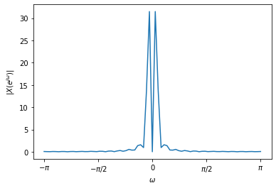
As you can see, some low frequency components (near zero) have large magnitudes. And there are small non-zero activations in other frequencies. You might ask: x consists of only one frequency (440Hz), why don’t we see only one (actually two, it should be symmetric around zero) non-zero components? This would be true it x was periodic but it is not. It is not periodic because it does not extend to minus infinity to plus infinity. It is a time-limited signal. Due to this time-limited nature, we see many frequency components to have non-zero magnitudes.

Let us also have a look at the magnitude spectrums of the noise.

Xn,magn,w = dtft(noise)
fig = plt.figure()
plt.plot(w,magn)
plt.xlabel(r'$\omega$')
plt.ylabel(r'$|X_{noise}(e^{j\omega})|$');
fig.axes[0].set_xticks([-np.pi, -np.pi/2, 0, np.pi/2, np.pi])
fig.axes[0].set_xticklabels([r'$-\pi$', r'$-\pi/2$', 0, r'$\pi/2$', r'$\pi$']);

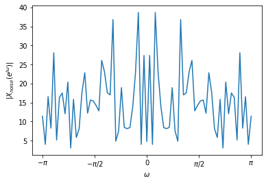
It has non-zero magnitudes all over the frequency domain. This is due to the standard normal noise. Let us look at the spectrum of only the high-pitch tone.

hp = 0.5*np.sin(noise_freq * 2 * np.pi * n) 
Xhp,maghp,w = dtft(hp)
fig = plt.figure()
plt.plot(w,maghp)
plt.xlabel(r'$\omega$')
plt.ylabel(r'$|X_{high-pitch}(e^{j\omega})|$');
fig.axes[0].set_xticks([-np.pi, -np.pi/2, 0, np.pi/2, np.pi])
fig.axes[0].set_xticklabels([r'$-\pi$', r'$-\pi/2$', 0, r'$\pi/2$', r'$\pi$']);

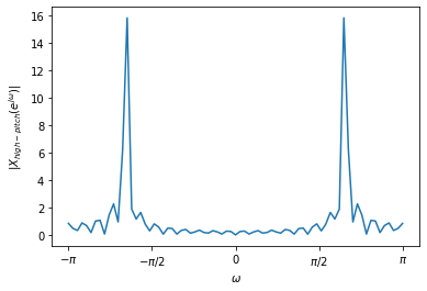
This plot clearly shows two high-frequency (around 2 and -2) components having large magnitudes. And, here is the spectrum of the polluted signal y.

Y,magy,w = dtft(y)
fig = plt.figure()
plt.plot(w,magy)
plt.xlabel(r'$\omega$')
plt.ylabel(r'$|Y(e^{j\omega})|$');
fig.axes[0].set_xticks([-np.pi, -np.pi/2, 0, np.pi/2, np.pi])
fig.axes[0].set_xticklabels([r'$-\pi$', r'$-\pi/2$', 0, r'$\pi/2$', r'$\pi$']);

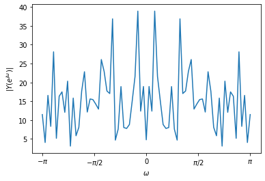
Remember that our goal was to recover x from y. Looking at the Fourier transform specrum of y above, it does not look possible to discern the contributions of x and y in this plot.

To tackle this problem, we wil introduce the Discrete Fourier Transform (DFT), which is specially designed to analyze time-limited signals, such as x.

Discrete Fourier Transform (DFT)

The DFT computes frequency coefficients for a time-limited input signal, whose samples are equally spaced apart. The following is the analysis equation of DFT:

\[ X_k = \sum_{n=0}^{N-1} x[n] e^{-j 2 \pi \frac{k}{N} n}. \]

Compare this to the analysis equation of DTFT:

\[ \quad X(e^{j\omega}) = \sum_{n=-\infty}^{\infty}x[n]e^{-j\omega n}. \]

The major difference between the two is that in DFT, the sum runs from 0 to N (hence, time-limited). And, the DFT returns a sequence of complex numbers (\(X_k\)) but the DTFT returns a complex-valued continuous function (\(X(e^{j\omega})\)).

At this point, it should be trivial to implement the analysis equation of DFT. We leave this as an exercise for the reader. Numpy provides a function to compute DFT. In the following, we will use numpy’s fft to compute the DFT.

Let us compute and plot the DFT of x, the pure A4 tone.

Xk = np.fft.fft(x)
freq = np.fft.fftfreq(n.shape[-1])
plt.plot(freq, np.abs(Xk))
plt.xlabel('k/N')
plt.ylabel(r'$|X_k|$');

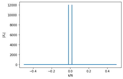
As you can see, there are two large magnitude components for a certain low frequency (around 0, for +k and -k). And now, let us observe the DFT magnitude spectrum of the noise.

sp = np.fft.fft(noise)
freq = np.fft.fftfreq(n.shape[-1])
plt.figure(), plt.plot(freq, np.abs(sp));
print(np.abs(sp[:100]))

[26.3939262  19.78082531 18.5613526  18.16154192 12.85042881  3.94131067
 16.50537601 11.43596066  8.93393148 27.84900581 17.75504459 15.2950187
  7.49519863  0.68329369 24.85026763 12.22252806 10.84516839  3.91734097
  4.60748016 11.14280738 11.59918517 15.30721717 11.76383234 21.76361059
  6.97365424 14.81363106 10.27026245 18.1318892  11.03912535 11.69918618
 17.4346365  26.34435528 14.97047224 12.77150336  4.19053788 12.60260081
  3.31775452 17.6138151  10.54790777  9.20298745  9.21247828 15.43979215
 26.34879589 24.27338127 12.12848432  5.18655424  3.98540724 15.39359425
 19.6169026  14.60770132 13.49198957 16.41172377 12.80964137 13.00230983
 10.28430403 18.96414161 24.1202784   7.61211008 11.4995437  15.87033274
 16.61097415  6.76293908 14.20044128  5.16949221 11.7284264  14.4083265
 18.83707131 15.8498208   3.81093534  4.59328883  3.93130371 21.55730351
 22.52954596  9.62680013 12.44274316  9.87832883  8.67612092 16.13511936
 12.86832829 14.76306173 20.86812966 22.93384788  2.94799523 18.28669552
  8.11635209 27.13605712 10.61571555 12.14065374  7.93123885 11.35498035
 15.99021726  6.02722655 10.88325072 10.71628915 13.89580347 15.85038919
  3.30288681 23.78253858 21.30445441 14.19958133]

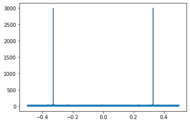
The noise is characterised by two large magnitude high frequency components. And also, small but non-zero magnitudes all over the spectrum, as printed above. The DFT magnitude spectrum of y is as follows.

Yk = np.fft.fft(y)
freq = np.fft.fftfreq(n.shape[-1])
plt.figure(), plt.plot(freq, np.abs(Yk));
plt.xlabel('k/N')
plt.ylabel(r'$|Y_k|$');

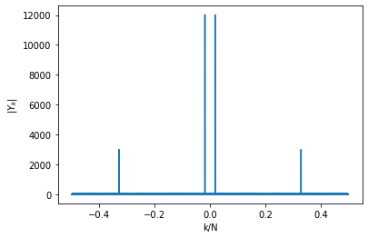
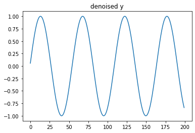
This plot clearly shows that y consists of one low frequency and one high frequency component. To keep the low frequency component only, we can zero out everything that has a magnitude less than 3000. Below we do this modification and reconstruct back the signal using inverse DFT, which should remove the noise in y. You can find the plot of denoised y (compare this with the original plot of y at the beginning of this notebook) and listen to it. It should sound like the pure A4 tone you listenede to above.

Yk[np.abs(Yk)<3000] = 0

x_recons = np.real(np.fft.ifft(Yk))
plt.plot(np.real(x_recons[:200]))
plt.title('denoised y')

sd.default.reset()
sd.play(np.real(x_recons), sampleRate)